← Previous Topic: Why Mathematical Modeling?.

Classical Modal Analysis

For linear systems, modal analysis is an elegant blend of quantitative and qualitative techniques. It accurately predicts linear system response, but also characterizes the general behavior of the linear system. Modal analysis is built on simple idea - find a new coordinate system where the original system has a simpler form that is easier to understand. It turns out that for linear systems, where the linear coefficients are constant, there is always a coordinate system where the system of ODEs has a simple form called the Jordan cannonical form. In many cases, when coordinates are selected such that the system is in Jordan cannonical form, all of the ODEs in the system are decoupled, which means they can be solved independently. In some cases, referred to as degenerate cases, there is a simple coupling between some of the ODEs in the system. Only the more common nondegenerate cases are discussed below.

Example System

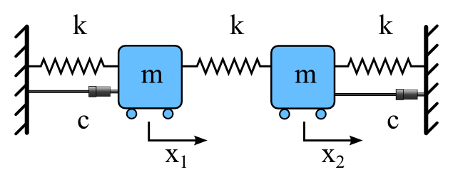
As an example consider a linear two mass system with springs connecting the masses to each other an to the walls, and a damper between each mass and the wall. To model the system, Newtons law ($F=ma$) can be applied to a free body diagram of each of the masses. The equations for the masses are:

$m{d^2x_1}/{dt^2} = -c{dx_1}/{dt} - k x_1 + k(x_2-x_1)$
$m{d^2x_2}/{dt^2} = -c{dx_2}/{dt} - k x_2 + k(x_1-x_2)$

If this is simplified by assuming that the spring constant (k) and the damper constant (c) each have a value of 1, and that the mass (m) is small enough to be ignored, then the following system of equations predicts the motion of the two masses:

${dx_1}/{dt} = -2 x_1 + x_2$
${dx_2}/{dt} = x_1 - 2 x_2$

For the system, both $x_1$ and $x_2$ change with $t$ (which in this system represents time). This is a coupled system because the change in $x_1$ with respect to $t$ depends on the value of both $x_1$ and $x_2$. Similarly, the change in $x_2$ with respect to $t$ depends on both $x_1$ and $x_2$. Since the equations depend on one another, both must be solved simultaneously.

If the terms $a_{ij}$ are constants, a linear change of coordinates has the form:

$q_1 = a_{11} x_1 + a_{12} x_2$
$q_2 = a_{21} x_1 + a_{22} x_2$

With the right choice of coordinates, the system above can be represented in the uncoupled form:

${dq_1}/{dt} = -q_1$
${dq_2}/{dt} = -3 q_2$

In this form, the change in $q_1$ with respect to $t$ only depends on $q_1$ so this can be solved independent of $q_2$. Similarly, the change in $q_2$ with respect to $t$ only depend on $q_2$ so this can be solved independent of $q_1$.

What is Model Analysis

Modal Analysis the process of finding the linear choice of coordinates where the ODEs of the system are decoupled from one another. The new coordinates are called modal coordinates.

For linear systems, the quantitative accuracy of modal analysis comes from the fact that the new modal system is the same as the original system, or in other words no approximation is required. The only difference is the coordinate system that is used. The qualitative understanding comes from the fact that modal analysis converts coupled ODEs that are typically too complex to understand as a whole, because the solutions are intertwined, to a decoupled set of ODEs which are simpler to understand because the modal ODEs can be solved and explored independently. The modal solutions can be added (or superimposed) to get the total system response. The power of modal analysis comes from the fact that you can understand the total behavior of the system in terms of the individual behavior of the modes.

For nonlinear systems, there is often a region around an equilibrium or steady state solution were a linear system of ODEs provides a good approximation and modal analysis gives reasonably accurate results. However, there are many cases where a linear approximation misses important trends, and cases where the response grows to the point where nonlinear terms are important, and modal analysis gives poor results. So while modal analysis will remain an important tool for the study of linear and nonlinear systems, there is a need to generalize the approach so that the elegant blend of quantitative and qualitative analysis are preserved.

Calculating the Modal Equations

First Order Form

Before generalizing modal analysis to nonlinear systems, lets take a look at how modal coordinates, which decouple a linear system of ODEs, are calculated for linear systems. We will start with a system of ODEs expressed as a matrix in first order form. This is a way of representing the system of ODEs where only first order derivatives are part of the system of ODEs. Click here for a discussion of how to convert a system with higher order derivates to first order form. A linear system in first order form, with no forcing terms can be written like:

(1)    ${dx_i}/{dt} = A_{ij} x_j$

As noted above, in order for modal analysis to work, the value of the coefficients in $A_{ij}$ must not change with $t$. In other words, the coeffients can be constant values, or constant parameters such as a mass or stiffness quantity, but can't depend on $t$ (or $x_1, x_2, ..., x_n$, since these values change with $t$). We will explain why the coefficients can't be dependent on $t$ in the discussion below. The linear modal coordinate function $q$ can be written in the form:

(2)    $q = c_i x_i = c_1 x_1 + c_2 x_2 + ... + c_n x_n$

where $c_i$ is a vector with values that do not depend on $t$.

Example System

Consider the example system shown above:

${dx_1}/{dt} = -2 x_1 + x_2$
${dx_2}/{dt} = x_1 - 2 x_2$

In Matrix Form this is represented as:

$(\table {dx_1}/{dt}; {dx_2}/{dt}) = (\table -2, 1; 1, -2) (\table x_1; x_2)$

The modal coordinate function in matrix form is written as:

(3)    $q = (\table c_1, c_2) (\table x_1; x_2) = c_1 x_1 + c_2 x_2$

To calculate a modal coordinate of a system of ODEs, we do the following:

Step 1 - Calculate an Eigenvector

The first step for determining a modal coordinate is to calculate a left eigenvector $c_i$. A left eigenvector a vector that solves the equation:

(4)    $c_i A_{ij} = λ c_j$

This is called a left eigenvector because it is an eigenvector calculated by multiplying the matrix $A_{ij}$ by a row vector $c_i$ on the left side.

Step 1 Example

For the example system above the left eigenvector equation is:

$(\table c_1, c_2) (\table -2, 1; 1, -2) = λ (\table c_1, c_2)$

The associated algebraic equations are:

$-2 c_1 + c_2 =$	$λ c_1$
$c_1 - 2 c_2 =$	$λ c_2$

Modes of the Example System

The above algebraic equations have two (modal coordinate) solutions which can be found with a little algebra:

---

Mode 1

$λ = -1$ and $(\table c_1, c_2) = (\table s, s)$ where $s$ is a real number. From this we get $q_1 = s x_1 + s x_2$

---

Mode 2

$λ = -3$ and $(\table c_1, c_2) = (\table s, -s)$ where $s$ is a real number. From this we get we get $q_2 = s x_1 - s x_2$

---

For modal analysis, the arbitrary constant $s$ is typically set of some specific value such as 1. However, we will just keep the constant $s$ below since it helps identify where our modal coordiantes have been substituted.

Step 2 - Left Multiply the System of ODEs by the Eigenvector

Left multiplying the system of ODEs from equation (1) by the eigenvector $c_i$ and applying the eigenvector equation from (4) gives:

(5)    $c_i {dx_i}/{dt} = c_i A_{ij} x_j = λ c_i x_i$

Step 2 Example

---

Mode 1

$(\table s, s) (\table {dx_1}/{dt}; {dx_2}/{dt}) = -1 (\table s, s) (\table x_1; x_2)$

---

Mode 2

$(\table s, -s) (\table {dx_1}/{dt}; {dx_2}/{dt}) = -3 (\table s, -s) (\table x_1; x_2)$

---

Step 3 - Bring the Left Hand Side Eigenvector inside the Derivative

Since the coefficient in $c_i$ are contant relative to $t$, we can insert $c_i$ into the differential on the left hand side of the equation. This is important because it results in the produce $c_i x_i$ inside the differential, which equals $q$ [see equation (2)].

(6)    ${d(c_i x_i)}/{dt} = λ c_i x_i$

Step 3 Example

---

Mode 1

${d}/{dt} ((\table s, s) (\table x_1; x_2)) = -1 (\table s, s) (\table x_1; x_2)$    ⇒    ${d}/{dt} (s x_1 + s x_2) = -1 (s x_1 + s x_2)$

---

Mode 2

${d}/{dt} ((\table s, -s) (\table x_1; x_2)) = -3 (\table s, -s) (\table x_1; x_2)$    ⇒    ${d}/{dt} (s x_1 - s x_2) = -3 (s x_1 - s x_2)$

---

Step 4 - Substitute in the Modal Coordinate

Both the left and right hand side of equation (6) now contain the product $c_i x_i$. From equation (2) this can be replaced by $q$ to get the decoupled modal ODE:

(7)    ${dq}/{dt} = λ q$

Step 4 Example - Modal Equations

---

Mode 1

${dq_1}/{dt} = -q_1$

---

Mode 2

${dq_2}/{dt} = -3 q$

---

The Solution

The solution of the modal equation is $q = C e^{λ t}$ where $C$ is an arbitrary constant determined by initial conditions.

Solution for the Example Problem

---

Mode 1

$q_1 = C_1 e^{-t}$

---

Mode 2

$q_2 = C_2 e^{-3t}$

---

Nonlinear Systems

The modal analysis steps outlined above do not result in a decoupled ODE for nonlinear systems. The problem is that some of the coefficients in the matrix $A_{ij}$ will be functions of $x_1, x_2, ..., x_n$. This means the eigenvectors will also depend on these variables. Since $x_1, x_2, ..., x_n$ change with $t$, the eigenvectors $c_i$ have a dependence on $t$, and the process fails at step 3 because a terms that changes with $t$ can't be brought inside the derivative term. Since we can't bring $c_i$ inside the derivative, we don't have the product $c_i x_i$ on the left hand side of the equation, so we can't replace the $c_i$ and $x_i$ with $q$, and the process for decoupling the ODE fails.

So how do we fix this issue for nonlinear systems? Well, it turns out that for linear systems, the step shown above are a combination of the chain rule along with a decoupling condition, although this isn't obvious. The chain rule is the general rule for applying a change of coordinates to any system of ODEs - linear or nonlinear. The problem is that the steps above are not consistent with the chain rule when we are dealing with a nonlinear system. In order to generalize modal analysis to nonlinear systems, the change of coordinates and the decoupling condition should be expressed in a form that is consistent with the chain rule.

Next Topic - Extending Modal Analysis to Nonlinear Systems